SciencePlots Basics and Features

August 26, 2023 · 6 min read

If you have any questions, feel free to comment below. Click the block can copy the code.
And if you think it's helpful to you, just click on the ads which can support this site. Thanks!

Users sometimes need to customize layer properties such as fonts, tick axes, spines, and legends according to a journal’s figure-drawing requirements, which is time-consuming and can also easily cause users to overlook some layer-detail requirements.

As a third-party extension toolkit specifically for drawing scientific-paper figures, SciencePlots provides Matplotlib plot styles (Matplotlib Styles) for mainstream English-language scientific journals (such as Nature, Science, and IEEE).

The installation code for SciencePlots is as follows:

pip install SciencePlots

Installing LaTeX #

To better display academic-paper illustrations and facilitate subsequent printing, the font style in illustrations is generally required to be a LaTeX typesetting style, and SciencePlots can easily meet this requirement. For the SciencePlots library to implement a LaTeX typesetting style, users need to install LaTeX on their computers.

For installation steps on other types of operating systems, simply refer to the official SciencePlots tutorial.

Install MikTex and Ghostscript The official ScienePlots library recommends that users install LaTeX using MikTex software. Users can directly download its latest version from the official MikTex website and install it. Ghostscript is a set of free software compiled based on Adobe, PostScript, portable document format (PDF) page-description languages, and so on. Users can download the latest version from its official website and install it.
Add the software installation paths to the system environment variables After installing the above two software packages, users also need to add their installation paths to the system environment variables, specifically “\...\miktex\bin\x64” and “\...\gs__(version number)\bin”. After adding the system environment variables, restart, and the relevant configuration will take effect.

SciencePlots Plotting Examples #

If the journal to which the reader is submitting has special font requirements, the reader can configure plotting without LaTeX:: plt.style.use(['science',' no-latex']).

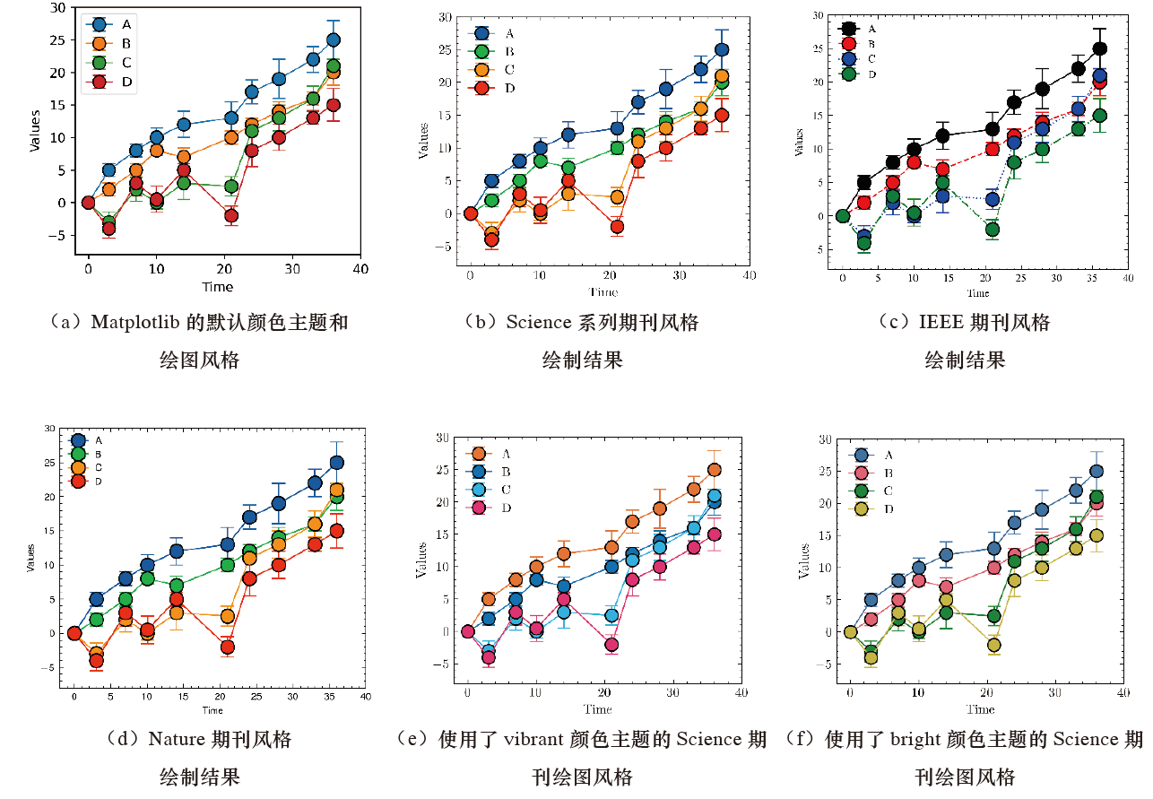
The figure below shows examples of several plotting styles in SciencePlots, (a) is Matplotlib’s default color theme and plotting style

import pandas as pd
import numpy as np
import matplotlib.pyplot as plt


data = pd.read_excel(r"\分组误差线图构建.xlsx")

#(a)Matplotlib's default color theme and plotting style
selsect = ["A","B","C","D"]
colors = ["#2FBE8F","#459DFF","#FF5B9B","#FFCC37"]
fig,ax = plt.subplots(figsize=(4,3.5),dpi=100,facecolor="w")

for index,color in zip(selsect,colors):
    data_selcet = data.loc[data['type']==index,:]
    ax.errorbar(x=data_selcet["time"],y=data_selcet["mean"],yerr=data_selcet["sd"],
                linewidth=1,marker='o',ms=10,mew=1,mec='k',capsize=5,label=index)
    ax.legend()
    ax.set(xlabel='Time', ylabel='Values',
           xlim=(-2,40),ylim=(-8,30))

plt.savefig('\第2章 绘制工具及其重要特征\图2-3-8 ScienecePlots_matplotlib.png', 
         bbox_inches='tight',dpi=600)
plt.savefig('\第2章 绘制工具及其重要特征\图2-3-8 ScienecePlots_matplotlib.pdf', 
         bbox_inches='tight') 
plt.show()

(b) is the result drawn in the style of the Science journal series

#(b)Result drawn in the style of the Science journal series

selsect = ["A","B","C","D"]
colors = ["#2FBE8F","#459DFF","#FF5B9B","#FFCC37"]
plt.style.use('science')
fig,ax = plt.subplots(figsize=(4,3.5),dpi=100,facecolor="w")
for index,color in zip(selsect,colors):
    data_selcet = data.loc[data['type']==index,:]
    ax.errorbar(x=data_selcet["time"],y=data_selcet["mean"],yerr=data_selcet["sd"],
                linewidth=1,marker='o',ms=10,mew=1,mec='k',capsize=5,label=index)
    ax.legend()
    ax.set(xlabel='Time', ylabel='Values',
           xlim=(-2,40),ylim=(-8,30))
plt.savefig('\第2章 绘制工具及其重要特征\图2-3-8 SciencePlots_science.png', 
         bbox_inches='tight',dpi=600)
plt.savefig('\第2章 绘制工具及其重要特征\图2-3-8 SciencePlots_science.pdf', 
         bbox_inches='tight') 
plt.show()

#(c)Result drawn in the IEEE journal style
selsect = ["A","B","C","D"]
colors = ["#2FBE8F","#459DFF","#FF5B9B","#FFCC37"]
plt.style.use(['science','ieee'])
fig,ax = plt.subplots(figsize=(4,3.5),dpi=100,facecolor="w")
for index,color in zip(selsect,colors):
    data_selcet = data.loc[data['type']==index,:]
    ax.errorbar(x=data_selcet["time"],y=data_selcet["mean"],yerr=data_selcet["sd"],
                linewidth=1,marker='o',ms=10,mew=1,mec='k',capsize=5,label=index)
    ax.legend()
    ax.set(xlabel='Time', ylabel='Values',
           xlim=(-2,40),ylim=(-8,30))
plt.savefig('\第2章 绘制工具及其重要特征\图2-3-8 SciencePlots_ieee.png', 
         bbox_inches='tight',dpi=600)
plt.savefig('\第2章 绘制工具及其重要特征\图2-3-8 SciencePlots_ieee.pdf', 
         bbox_inches='tight') 
plt.show()

(d) is the result drawn in the Nature journal style

#(d)Result drawn in the Nature journal style
colors = ["#2FBE8F","#459DFF","#FF5B9B","#FFCC37"]
selsect = ["A","B","C","D"]
plt.style.use(['science','nature'])
fig,ax = plt.subplots(figsize=(4,3.5),dpi=100,facecolor="w")
for index,color in zip(selsect,colors):
    data_selcet = data.loc[data['type']==index,:]
    ax.errorbar(x=data_selcet["time"],y=data_selcet["mean"],yerr=data_selcet["sd"],
                linewidth=1,marker='o',ms=10,mew=1,mec='k',capsize=5,label=index)
    ax.legend()
    ax.set(xlabel='Time', ylabel='Values',
           xlim=(-2,40),ylim=(-8,30))

plt.savefig('\第2章 绘制工具及其重要特征\图2-3-8 SciencePlots_nature.png', 
         bbox_inches='tight',dpi=600)
plt.savefig('\第2章 绘制工具及其重要特征\图2-3-8 SciencePlots_nature.pdf', 
         bbox_inches='tight') 
plt.show()

(e) is the Science journal plotting style using the vibrant color theme

#(e)Science journal plotting style using the vibrant color theme
selsect = ["A","B","C","D"]
plt.style.use(['science','vibrant'])
fig,ax = plt.subplots(figsize=(4,3.5),dpi=100,facecolor="w")
for index,color in zip(selsect,colors):
    data_selcet = data.loc[data['type']==index,:]
    ax.errorbar(x=data_selcet["time"],y=data_selcet["mean"],yerr=data_selcet["sd"],
                linewidth=1,marker='o',ms=10,mew=1,mec='k',capsize=5,label=index)
    ax.legend()
    ax.set(xlabel='Time', ylabel='Values',
           xlim=(-2,40),ylim=(-8,30))

plt.savefig('\第2章 绘制工具及其重要特征\图2-3-8 SciencePlots_vibrant.png', 
         bbox_inches='tight',dpi=600)
plt.savefig('\第2章 绘制工具及其重要特征\图2-3-8 SciencePlots_vibrant.pdf', 
         bbox_inches='tight') 
plt.show()

(f) is the Science journal plotting style using the bright color theme

#(f)Science journal plotting style using the bright color theme
selsect = ["A","B","C","D"]
plt.style.use(['science','bright'])
fig,ax = plt.subplots(figsize=(4,3.5),dpi=100,facecolor="w")
for index,color in zip(selsect,colors):
    data_selcet = data.loc[data['type']==index,:]
    ax.errorbar(x=data_selcet["time"],y=data_selcet["mean"],yerr=data_selcet["sd"],
                linewidth=1,marker='o',ms=10,mew=1,mec='k',capsize=5,label=index)
    ax.legend()
    ax.set(xlabel='Time', ylabel='Values',
           xlim=(-2,40),ylim=(-8,30))
           
plt.savefig('\第2章 绘制工具及其重要特征\图2-3-8 SciencePlots_bright.png', 
         bbox_inches='tight',dpi=600)
plt.savefig('\第2章 绘制工具及其重要特征\图2-3-8 SciencePlots_bright.pdf', 
         bbox_inches='tight') 
plt.show()

For more plotting styles, refer to the official SciencePlots website.

Tip: The SciencePlots library not only provides plotting-style templates for mainstream English-language scientific journals, but can also mix different plotting styles. In addition, when using the library’s plotting styles, readers can set the global plotting style through plt.style.use('science'), or temporarily use a plotting style through the following statement.

with plt.style.context('science '):
	plt.figure()
	plt.plot(x,y)
	plt.show()

Global settings are recommended because when using a temporary plotting style, especially when LaTeX characters are used, it will be impossible to use the LaTeX character style when drawing layer properties such as legends and axis labels, causing the overall plotting result to be uncoordinated. The method for introducing SciencePlots plotting theme styles may vary as versions are updated. Readers should check the official SciencePlots website and use its latest introduction method.