Python Data Manipulation

July 12, 2024 · 4 min read

If you have any questions, feel free to comment below. Click the block can copy the code.
And if you think it's helpful to you, just click on the ads which can support this site. Thanks!

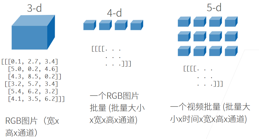
An $n$-dimensional array is also called a tensor. Regardless of the deep learning framework, its tensor class (ndarray in MXNet and Tensor in PyTorch and TensorFlow) is similar to NumPy’s ndarray. During deep learning training, we usually do not read images one at a time. Instead, we might read 128 images at once. This is a batch, represented by a four-dimensional array. Deep learning frameworks also offer important features beyond NumPy’s ndarray:

Strong support for GPU-accelerated computation, while NumPy supports only CPU computation;
Automatic differentiation in tensor classes.

A tensor with one axis corresponds to a mathematical vector; A tensor with two axes corresponds to a mathematical matrix.

Tensor Methods #

arange #

arange creates a row vector x containing the first 12 integers starting at 0.

x = torch.arange(12)
# tensor([ 0,  1,  2,  3,  4,  5,  6,  7,  8,  9, 10, 11])

shape #

Use the shape attribute to access a tensor’s shape (its length along each axis).

x.shape # torch.Size([12])

reshape #

Call reshape to change a tensor’s shape without changing its number of elements or their values.

X = x.reshape(3, 4)

You do not need to calculate every dimension exactly: use -1 to have one dimension inferred automatically. x.reshape(-1,4) or x.reshape(3,-1) can replace x.reshape(3,4).

zeros ones randn #

Initialize matrices with all zeros, all ones, other constants, or numbers randomly sampled from a specific distribution.

torch.zeros((2, 3, 4))
#tensor([[[0., 0., 0., 0.],
#         [0., 0., 0., 0.],
#         [0., 0., 0., 0.]],
#
#        [[0., 0., 0., 0.],
#         [0., 0., 0., 0.],
#         [0., 0., 0., 0.]]])
torch.ones((2, 3, 4))
# Randomly sample from a standard Gaussian (normal) distribution with mean 0 and standard deviation 1.
torch.randn(3, 4)
#tensor([[-0.0135,  0.0665,  0.0912,  0.3212],
#        [ 1.4653,  0.1843, -1.6995, -0.3036],
#        [ 1.7646,  1.0450,  0.2457, -0.7732]])

You can also create a tensor directly from a manually written list.

Operators #

Elementwise Operations #

Standard arithmetic operators (+, -, *, /, and **) can all be applied elementwise. We can perform elementwise operations on any two tensors of the same shape.

x + y, x - y, x * y, x / y, x ** y  # ** is exponentiation
torch.exp(x)

Linear Algebra Operations #

Concatenate multiple tensors along rows (axis 0, the first element of the shape) or columns (axis 1, the second element of the shape).

X = torch.arange(12, dtype=torch.float32).reshape((3,4))
Y = torch.tensor([[2.0, 1, 4, 3], [1, 2, 3, 4], [4, 3, 2, 1]])

torch.cat((X, Y), dim=0)
#(tensor([[ 0.,  1.,  2.,  3.],
#         [ 4.,  5.,  6.,  7.],
#         [ 8.,  9., 10., 11.],
#         [ 2.,  1.,  4.,  3.],
#         [ 1.,  2.,  3.,  4.],
#         [ 4.,  3.,  2.,  1.]]),

torch.cat((X, Y), dim=1)
# tensor([[ 0.,  1.,  2.,  3.,  2.,  1.,  4.,  3.],
#         [ 4.,  5.,  6.,  7.,  1.,  2.,  3.,  4.],
#         [ 8.,  9., 10., 11.,  4.,  3.,  2.,  1.]]))
X == Y
#tensor([[False,  True, False,  True],
#        [False, False, False, False],
#        [False, False, False, False]])
X.sum()
# tensor(66.)

Broadcasting #

Because a and b are $3\times1$ and $1\times2$ matrices, respectively, their shapes do not match for addition. We broadcast both matrices to a larger $3\times2$ matrix as follows: replicate the columns of a and the rows of b, then add them elementwise.

Indexing and Slicing #

Tensor elements can be accessed by index. The first element has index 0, and the last has index -1; a range includes its start but excludes its end (start-inclusive, end-exclusive). You can also assign values through indexing.

X[0:2, :] = 12
#tensor([[12., 12., 12., 12.],
#        [12., 12., 12., 12.],
#        [ 8.,  9., 10., 11.]])

Saving Memory #

Some operations allocate memory for a new result. For example, with Y = X + Y, Y stops referring to its previous tensor and instead points to a tensor in newly allocated memory.

The id() function gives us the identity of the object referenced in memory.

# After running `Y = Y + X`, we find that `id(Y)` refers to a different location.
before = id(Y)
Y = Y + X
id(Y) == before

This may be undesirable for two reasons:
First, we do not want to allocate memory unnecessarily. In machine learning, we may have hundreds of megabytes of parameters and update all of them multiple times per second. We generally want to perform these updates in place.
Without in-place updates, other references still point to the old memory location, so some code may inadvertently use outdated parameters.

You can use slice notation to assign the result of an operation to a previously allocated array, such as Y[:] = <expression>.

Z = torch.zeros_like(Y)
print('id(Z):', id(Z))
# A slice is a view.
Z[:] = X + Y
print('id(Z):', id(Z))

# id(Z): 137141768464768 
# id(Z): 137141768464768

Of course, this still allocates space for the extra variable Z. To reduce memory use further, use X as the result if it will not be needed later. Use X[:] = X + Y or X += Y to reduce the memory overhead of the operation.

Converting to Other Python Objects #

A torch tensor and a NumPy array can share underlying memory; changing one in place also changes the other.

A = X.numpy()
B = torch.tensor(A)
type(A), type(B)
# Convert a tensor with only one element to a scalar.
b = torch.tensor([6.6])
b, b.item(), float(b), int(b) 
# (tensor([6.6000]), 6.599999904632568, 6.599999904632568, 6)

Summary #

torch.arange()
x.shape()
x.reshape()
torch.ones() torch.zeros() torch.randn()
torch.tensor()
torch.cat((X, Y), dim=0)
X[0:2, :] = 6
X[:] = X + Y or X +=Y