Image Classification and Foundational Vision Models

March 7, 2022 · 3 min read

If you have any questions, feel free to comment below. Click the block can copy the code.
And if you think it's helpful to you, just click on the ads which can support this site. Thanks!

Process #

1. Collect data

2. Define the model

   Usually a function containing parameter variables: \(y=F_{\Theta}(X)\)

   Example: \(y=\sigma\left(\Theta^{T} X\right)\)

3. Train Find the optimal parameters \(\Theta^{*}\) so that the model \(y=F_{\Theta^{*}}(X)\) achieves the highest accuracy on the training set

4. Predict For a new image \(\hat{X}\) , use the trained model to predict its class, namely \(\hat{y}=F_{\Theta^{*}}(\hat{X})\)

Traditional Methods: Designing Image Features (1990s~2000s) #

The Ceiling of Feature Engineering #

In the ImageNet image recognition challenge, the champion teams in 2010 and 2011 both used classic vision methods, implementing image classification based on manually designed features + machine learning algorithms, with Top-5 error rates around 25%.

From Feature Engineering to Feature Learning #

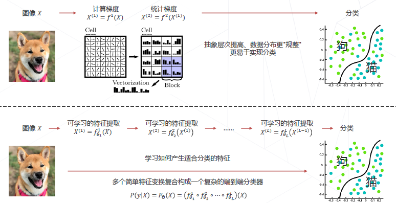
Ways to Implement Hierarchical Features #

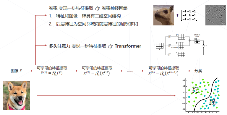
The Birth of AlexNet & the Beginning of the Deep Learning Era #

In the 2012 competition, a team from the University of Toronto used a deep learning method for the first time, reducing the error rate to 15.3% in one stroke, while the performance of traditional vision algorithms had already reached a bottleneck; in 2015, the performance of convolutional networks surpassed humans.

Mathematical Representation of Image Classification #

1. Model design: design \(𝐹_Θ 𝑋\) suitable for images • Convolutional neural networks • Lightweight convolutional neural networks • Neural architecture search • Transformer

2. Model learning: solve for a good set of parameters Θ • Supervised learning: learning based on labeled data • Loss functions • Stochastic gradient descent algorithms • Common training techniques for vision models • Self-supervised learning: learning based on unlabeled data

AlexNet (2012) #

The first model to successfully implement large-scale images, achieving a ~85% top-5 accuracy on the ImageNet dataset.

Characteristics:

• 5 convolutional layers and 3 fully connected layers, with a total of 60M learnable parameters
• Uses the ReLU activation function, greatly improving convergence speed
• Implemented and open-sourced cuda-convnet, making it practically possible to train large-scale neural networks on GPUs

Going Deeper (2012~2014) #

VGG-19 19 layers ImageNet Top-5 accuracy: 92.7%

GoogLeNet 22 layers ImageNet Top-5 accuracy: 93.4%

VGG (2014) #

Decomposes large-sized convolutions into multiple layers of 3×3 convolutions, providing the same receptive field, fewer parameters, more layers, and greater representational capacity.

1 layer of 5×5 convolution and 2 layers of 3×3 convolution have the same receptive field

• Number of network layers: 11, 13, 16, 19 layers
• 3×3 convolutions combined with 1-pixel boundary padding maintain spatial resolution
• Every few layers, doubles the number of channels and halves the resolution, generating features at higher levels of abstraction at 1/2 and 1/4 scales

GoogLeNet (Inception v1, 2014) #

• Formed by stacking Inception modules, with 22 learnable layers
• The final classification uses only a single fully connected layer, saving a large number of parameters
• Only 7M weight parameters (AlexNet 60M, VGG 138M)

Accuracy Degradation Problem #

After the number of model layers increases to a certain point, classification accuracy decreases instead of increasing

The counterintuitiveness of the experiment

When convolution degenerates into an identity mapping, the deep network is identical to the shallow network. Therefore, the deep network should have classification accuracy no worse than that of the shallow network.

Hypothesis: Although deep networks have the potential to achieve higher accuracy, conventional optimization algorithms have difficulty finding this better model. That is, having the newly added convolutional layers fit an approximate identity mapping happens to make the shallow network a little better

Basic Idea of Residual Learning #

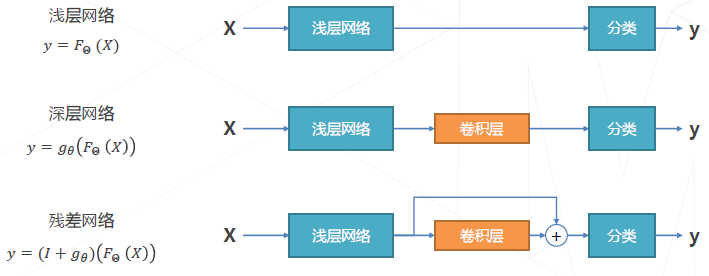
Residual modeling: let the newly added layers fit the difference between the shallow network and the deep network, which is easier to learn. Gradients can be directly propagated back to the shallow network to supervise its learning. No additional inputs are introduced, allowing parameters to contribute more effectively to the final model

Residual Network ResNet (2015) #

ResNet-34 34 layers ImageNet Top-5 accuracy: 94.4%

5 stages, each containing several residual modules; different numbers of residual modules produce different ResNet structures

• At each stage, the output resolution is halved and the number of channels is doubled
• Global average pooling compresses the spatial dimensions
• A single fully connected layer produces class probabilities

Use bottleneck modules to replace basic modules, further increasing the number of residual modules in each stage.

• ResNet-50 3/4/6/3 94.8% / 76.6%
• ResNet-101 3/4/23/3 95.4% / 78.0%
• ResNet-152 3/8/36/3 95.5% / 78.5%

Two Types of Residual Modules in ResNet #

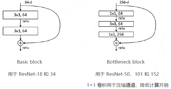
ResNet is equivalent to a multi-model ensemble: a residual network has \(𝑂(2^𝑛)\) implicit paths connecting the input and output, and each added block doubles the number of paths.

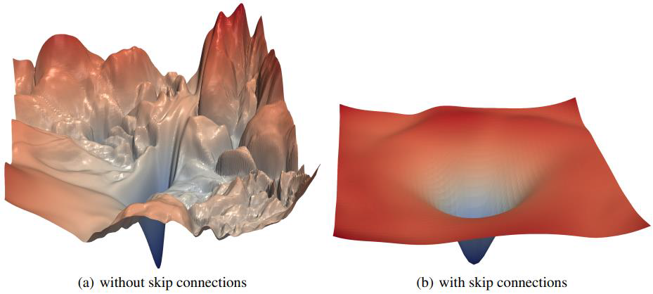
Residual Connections Make the Loss Surface Smoother #

The Loss Surface is smoother, making it easier to converge to a local/global optimal solution

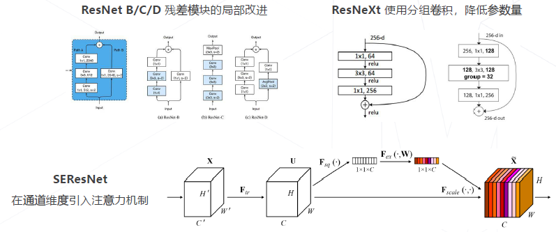
Subsequent Improvements to ResNet #