Numerical Descriptive Analysis

August 20, 2023 · 4 min read

If you have any questions, feel free to comment below. Click the block can copy the code.
And if you think it's helpful to you, just click on the ads which can support this site. Thanks!

Before the analysis, first convert the categorical variables low, race, smoke, ht, and ui in the birthwt dataset into factors.

library(MASS)
data(birthwt)
str(birthwt)

options(warn=-1)
library(dplyr)
birthwt <- birthwt %>% 
  mutate(low = factor(low, labels = c("no", "yes")),
         race = factor(race, labels = c("white", "black", "other")),
         smoke = factor(smoke, labels = c("no", "yes")),
         ht = factor(ht, labels = c("no", "yes")),
         ui = factor(ui, labels = c("no", "yes")))
str(birthwt)

Obtaining commonly used statistics for each variable in a data frame is a way to quickly explore a dataset, and this can be accomplished with the following command.

summary(birthwt)

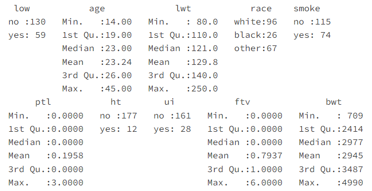
The summary( ) function can produce summary statistics for each variable. For numerical variables such as age, lwt, plt, ftv, and bwt, the summary( ) function gives the minimum, lower quartile, median, mean, upper quartile, and maximum; for categorical variables such as low, race, smoke, ht, and ui, it gives frequency tables.

Applying the summ( ) function from the epiDisplay package to a data frame produces summary output in another format. It arranges variables by row and places the minimum and maximum in the last two columns to make it convenient to view the range of the data.

library(epiDisplay)
summ(birthwt)

It should be noted that, for factor variables, the summ( ) function treats each level of the variable as a numerical value when calculating statistics.

4.1 Descriptive Statistical Analysis of Numerical Variables #

This section will discuss the central tendency, dispersion, and distribution shape of numerical variables. Here we focus on three continuous variables: age (age), the mother’s weight before pregnancy (lwt), and the infant’s weight at birth (bwt).

cont.vars <- dplyr::select(birthwt, age, lwt, bwt)

Next, first calculate descriptive statistics for these three variables, and then examine the descriptive statistics grouped by the mother’s smoking status (smoke). Here smoke is a binary variable, and when converting it into a factor we already defined labels for its two levels: “no” and “yes”.

In addition to the summary( ) function mentioned above, R has many functions for calculating specific statistics (see Chapter 2). For example, calculate the sample size, sample mean, and sample standard deviation of the variable age:

length(cont.vars$age)
mean(cont.vars$age)
sd(cont.vars$age)

We can also use the sapply( ) function to simultaneously calculate a specified statistic for multiple variables in a data frame. For example, calculate the sample standard deviation of each variable in the cont.vars data frame:

sapply(cont.vars, sd)

The base package does not provide functions for calculating skewness and kurtosis. We can calculate them ourselves according to the formulas, or call functions in other packages, such as the Hmisc, psych, and pstecs packages. These packages provide a wide variety of functions for calculating statistics, and they need to be installed before they are used for the first time. The psych package is used below as an example. The psych package is widely used in psychometrics.

The describe( ) function in the psych package can calculate the sample size after missing values are ignored, mean, standard deviation, median, trimmed mean, median absolute deviation, minimum, maximum, range, skewness, kurtosis, standard error of the mean, and other statistics for variables.

For example:

R.Version()
library(psych)
describe(cont.vars)

In many cases, we also want to calculate statistics for each category of a categorical variable. There are many ways to accomplish this task in R. The aggregate( ) and tapply( ) functions from the base package are introduced first below.

aggregate(cont.vars, by = list(smoke = birthwt$smoke), mean)
aggregate(cont.vars, by = list(smoke = birthwt$smoke), sd)

The by argument in the aggregate( ) function must be set to list. If list(birthwt$smoke) is used directly, the name of the grouping column above will be “Group.1” rather than “smoke”. We can also set multiple categorical variables inside list, for example:

aggregate(cont.vars, 
          by = list(smoke = birthwt$smoke, race = birthwt$race), 
          mean)

There are two categorical variables here: smoke has two categories and race has three categories. The command above calculates the mean for every combination of the categories of these two variables (six groups in total).

Of course, you can also write it in either of the following ways:

aggregate(birthwt[,c("age","lwt","bwt")], 
          by = list(smoke = birthwt$smoke, race = birthwt$race), 
          mean)

aggregate(cbind(age, lwt, bwt)~smoke+race, birthwt, mean)

The tapply( ) function can provide similar functionality. The difference is that its first argument must be a variable, and the name of its second argument is INDEX rather than by. For example, to calculate the mean of the variable bwt for different maternal smoking statuses, enter:

tapply(birthwt$bwt, INDEX = birthwt$smoke, mean)
# no 3055.69565217391 yes 2771.91891891892

The summ( ) function in the epiDisplay package can also provide similar functionality. The difference is that the statistics in this function are fixed, and the function’s output includes an ordered dot plot drawn according to the categorical variable, as shown below.

summ(birthwt$bwt, by = birthwt$smoke)

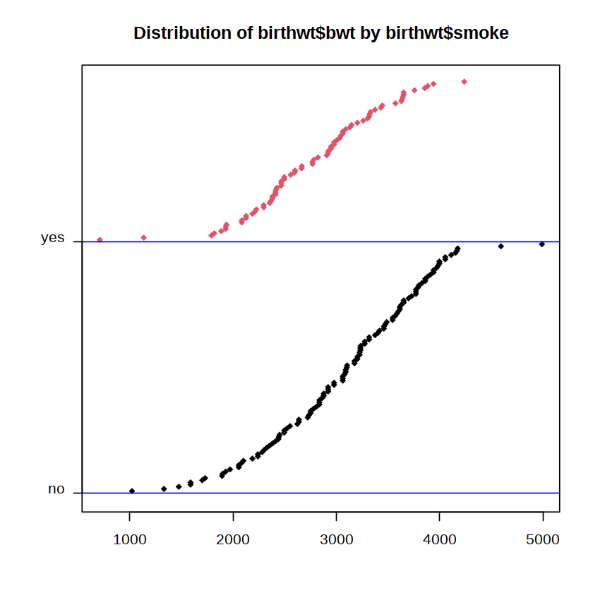
The ordered dot plot output by the summ( ) function is very convenient for exploring the distribution of numerical variables, especially the concentration trends and outliers in the data.

The describeBy( ) function in the psych package can also calculate the same statistics as the describe( ) function by group, for example:

describeBy(cont.vars, birthwt$smoke)

Although the describeBy( ) function is very convenient, it cannot specify arbitrary functions, so it has relatively poor extensibility. In fact, the group_by( ) and summarise( ) functions in the dplyr package introduced in Chapter 3 can calculate grouped statistics very flexibly. For example:

library(dplyr)
birthwt %>%
  group_by(smoke) %>% 
  summarise(Mean.bwt = mean(bwt), Sd.bwt = sd(bwt))

Data analysts can choose the method they are most accustomed to for calculating and presenting descriptive statistics. The last method has the clearest approach and the most concise results.

Numerical Descriptive Analysis

August 20, 2023 · 4 min read

4.1 Descriptive Statistical Analysis of Numerical Variables #

Related readings