Handling Missing Values

August 19, 2023 · 8 min read

If you have any questions, feel free to comment below. Click the block can copy the code.
And if you think it's helpful to you, just click on the ads which can support this site. Thanks!

Handling Missing Values #

In actual data analysis, missing data are frequently encountered. Missing values usually occur because data were not collected or were not entered.

For example, a missing age may be due to someone not providing his (her) age. Most statistical analysis methods assume that complete datasets are being processed. Therefore, apart from some specialized books, most statistics textbooks rarely address this issue. In fact, before conducting a formal analysis, we need to check whether the dataset contains missing values during the data preparation stage and use some methods to compensate for the loss caused by missing values.

1. Identifying Missing Values #

In R, missing values are represented by NA, an abbreviation for “Not Available.” The function is.na( ) can be used to identify missing values, and its return result is the logical value TRUE or FALSE.

height <- c(100, 150, NA, 160)
height
# 100 150 <NA> 160
is.na(height)
# FALSE FALSE TRUE FALSE

If there are few data, the number of missing values can be counted directly. For example, the variable height above has only one missing value. However, if the amount of data is large, the function table( ) is needed.

table(is.na(height))
# FALSE  TRUE 
#    3     1

It should be noted that the result of any calculation containing NA is NA. For example:

mean(height)
#  <NA>

To obtain the mean of all elements that can participate in the calculation, NA should first be removed from the vector.

mean(height, na.rm = TRUE)
# 136.666666666667

The parameter na.rm means removing missing values, and its meaning is the same as omitting missing values with the function na.omit( ).

mean(na.omit(height))

Note that na.omit( ) here is an independent function that can ignore missing values in the input object, whereas na.rm is only an internal parameter in functions that calculate descriptive statistics.

The function summary( ) automatically ignores missing values when calculating statistics for a vector, and it gives the number of missing values in the vector. For example:

summary(height)
#    Min. 1st Qu.  Median    Mean 3rd Qu.    Max.    NA's 
#   100.0   125.0   150.0   136.7   155.0   160.0       1

2. Exploring Missing Values in a Data Frame #

Before deciding how to handle missing values, it is very meaningful to understand which variables have missing values, how many there are, what combination patterns they have, and so on. The following example introduces methods for exploring missing-value patterns.

The dataset iris in the datasets package, also known as the iris flower data, contains 150 iris flower samples divided into 3 species (Species), with 50 samples of each species. Each sample also contains 4 attributes: sepal length (Sepal.Length), sepal width (Sepal.Width), petal length (Petal.Length), and petal width (Petal.Width). This dataset contains no missing values. To illustrate methods for handling missing values, some missing data are first generated artificially to explore missing-value patterns and test the effectiveness of imputation.

The function prodNA( ) in the missForest package can randomly generate missing values. The missForest package needs to be installed and loaded before using this function.

options(warn=-1)
library(missForest)
data(iris)
# To make the results reproducible, we use the function `set.seed( )` to set the seed for random-number generation.
set.seed(1234)
# By default, the function prodNA( ) generates missing values amounting to 10% of the data; we can generate different numbers of missing values by changing the value of the parameter noNA.
iris.miss <- prodNA(iris)
summary(iris.miss)

The number of missing values in each variable can be seen from the output of the function summary( ). To understand the patterns of missing values in a dataset, graphical display is a good approach. The VIM package provides a large number of functions for visualizing missing values. Among them, the function aggr( ) not only displays the number (or proportion) of missing values in each variable, but also displays the number (or proportion) of missing values under combinations of multiple variables. For example:

library(VIM)
aggr(iris.miss, prop = FALSE, numbers = TRUE, cex.axis = 0.7)

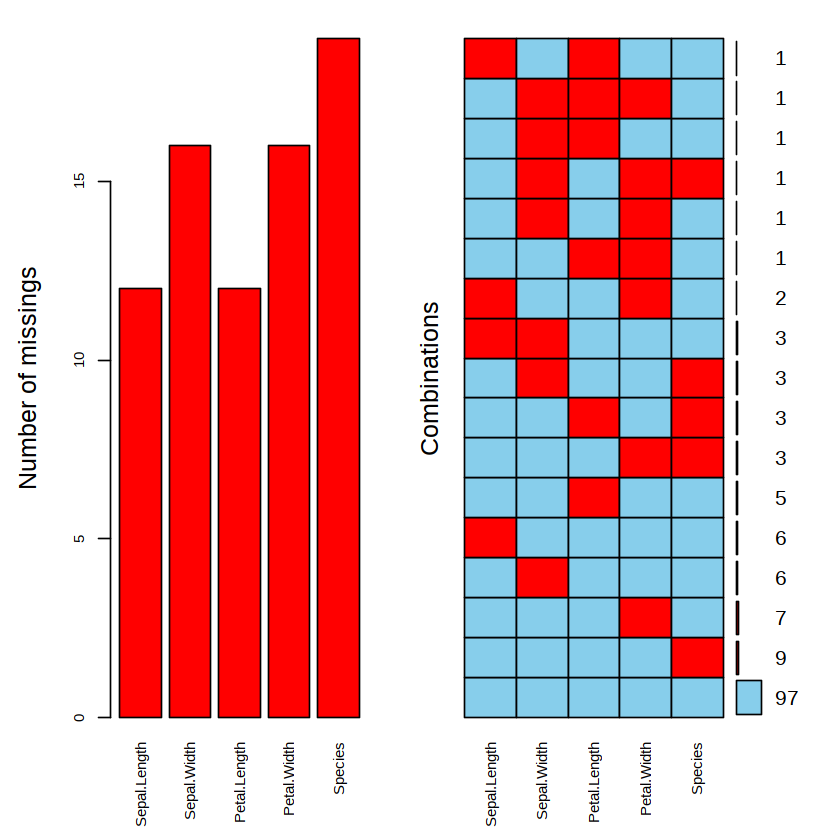
In the figure above, the first plot uses a bar chart to display the number of missing values in each variable, which is consistent with the output of the function summary( ) above; the second plot displays the number of missing values under different combinations of the 5 variables in the data frame, where red squares represent missing values and the numbers on the far right represent counts. Starting from the bottom, a total of 97 iris flower samples have no missing values, and 9 iris flower samples have all 4 of their attributes known but their species unknown.

3. Filling Missing Values #

Generally speaking, the following 3 methods can be used to handle missing values:

Deletion: delete variables or records with missing values;
Replacement: replace missing values with the mean, median, mode, or other values;
Imputation: infer and supplement missing values based on statistical models.

The methods above are all used only when there is no alternative. No method can completely compensate for the information loss caused by missing data. Therefore, missing data must be avoided as much as possible during the data collection stage.

3.1 Deleting Missing Values: na.omit( ), complete.cases( ) #

If the number of missing values is very small and deleting them has little effect on the analysis results, we can use the previously mentioned function na.omit( ) to delete missing values from a data frame. For example:

iris.sub <- na.omit(iris.miss)
nrow(iris.sub)

After deleting missing values, the data frame iris.sub contains only 97 complete records. In addition, the function complete.cases( ) can be used to identify rows in a matrix or data frame that have no missing values, and its return value is TRUE or FALSE. If a row has complete data, it returns TRUE; if a row contains at least one missing value, it returns FALSE. Therefore, the command above is equivalent to:

iris.sub <- iris.miss[complete.cases(iris.miss), ]

3.2 Replacing Missing Values with Specific Values #

If you do not want to delete missing values directly, in some cases you can also try replacing missing values with specific values. The following uses the variable Sepal.Length as an example, replacing the missing values in this variable with the mean after ignoring missing values. First calculate the mean:

Sepal.Length.Mean <- mean(iris.miss$Sepal.Length, na.rm = TRUE)
Sepal.Length.Mean
# 5.78695652173913
# Replace the missing values in this variable with the mean after ignoring missing values
iris.miss1 <- iris.miss
iris.miss1$Sepal.Length[is.na(iris.miss1$Sepal.Length)] <- Sepal.Length.Mean

To check the difference between the imputed data and the original data, we can calculate the deviation:

summary((iris$Sepal.Length - iris.miss1$Sepal.Length)/iris$Sepal.Length)
#  Min. 1st Qu. Median Mean 3rd Qu. Max.
# -0.258034 0.000000 0.000000 0.006871 0.000000 0.248447

The average deviation of the imputation is less than 1%, but the maximum deviation is approximately ±25%.

3.3 Multiple Imputation #

Multiple imputation is a method for handling missing values based on repeated simulation and is often used to handle relatively complex missing-value problems.

There are multiple packages in R that can perform multiple imputation of missing values, such as the Amelia package, mice package, and mi package. Among them, the mice package uses multivariate imputation by chained equations and is widely used in the data-cleaning process.

The mice package assumes that data are missing at random and builds models according to variable types to obtain predicted values to replace missing values. Commonly used among these models are:

Predictive mean matching^[1] (pmm), which is essentially linear regression and is suitable for numeric variables;
Logistic regression^[2] (logreg), which is suitable for binary variables;
Multinomial logistic regression^[3] (ployreg), which is suitable for unordered multicategorical variables;
Proportional odds model^[4] (polr), which is suitable for ordered multicategorical variables.

Next, use the function mice( ) to impute the missing values in the data frame iris.miss.

library(mice)
imputed.data <- mice(iris.miss, seed = 1234)
summary(imputed.data)
# PredictorMatrix:
#             Sepal.Length Sepal.Width Petal.Length Petal.Width Species
# Sepal.Length            0           1            1           1       1
# Sepal.Width             1           0            1           1       1
# Petal.Length            1           1            0           1       1
# Petal.Width             1           1            1           0       1
# Species                 1           1            1           1       0

In the matrix PredictorMatrix in the output above, each row represents the name of a variable containing missing values. If an element in a column corresponding to that row is 1, it means that the variable in that column was used for modeling and prediction.

It can be seen from the output above that, for each variable, all other variables were used to predict its missing values. The output of the function mice( ) is a list, and the object imp within it is also a list that stores the imputed values for the missing values of each variable. For example, the imputed values for the variable Sepal.Length can be obtained using the following command:

imputed.data$imp$Sepal.Length

The function mice( ) is completed through Gibbs sampling^[5]. By default, 5 random samples are performed, so a total of 5 sets of imputed values are obtained. We can check whether the imputed values are reasonable by examining the output above, and then select one set for imputation.

For example, take the 3rd of the 5 sets of imputed values:

complete.data <- complete(imputed.data, 3)

To check the effectiveness of filling in missing values, for numeric variables, we can calculate the deviation between the imputed values and the original variable values.

Using the variable Sepal.Length as an example:

summary((iris$Sepal.Length-complete.data$Sepal.Length)/iris$Sepal.Length)
#       Min.    1st Qu.     Median       Mean    3rd Qu.       Max. 
# -0.1428571  0.0000000  0.0000000  0.0007643  0.0000000  0.0945946

The average deviation of the imputation is less than 0.1%, and the maximum deviation is approximately ±13%. Therefore, multiple imputation is more effective here than replacing missing values with the mean.

The last variable Species in the data frame is a factor and contains 19 missing values. To check the effectiveness of filling in missing values for this categorical variable, we can use the function table( ) to obtain a contingency table of the original variable and the imputed variable:

table(iris$Species, complete.data$Species)
#              setosa versicolor virginica
#  setosa         50          0         0
#  versicolor      0         50         0
#  virginica       0          1        49

This type of table is called a confusion matrix^[6] and is often used to evaluate the accuracy of model predictions. The numbers on the diagonal represent the number of cases where the predicted values and true values agree, and the numbers off the diagonal represent the number of cases where the predicted values and true values disagree.

It can be seen from the output above that the accuracy rate of the imputation for the 19 missing values of the variable Species is 100%.