Using the dplyr Package
August 18, 2023 · 9 min read
If you have any questions, feel free to comment below. Click the block can copy the code.
And if you think it's helpful to you, just click on the ads which can support this site. Thanks!
This package handles data frames more efficiently with a unified specification. ** The first parameter of all functions that process data frames in the dplyr package is the data frame name. **
Taking the birthwt dataset in the MASS package as an example, the following describes the use of commonly used functions in the dplyr package. This data set comes from a case-control study of risk factors for low birth weight in newborns. Start by loading the dataset and viewing its related information.
library(dplyr)
data(birthwt, package = "MASS")
# ??birthwt
A total of 189 subjects and 10 variables were included in the dataset birthwt. where the outcome variable bwt is the weight of the newborn (unit: g) and the variable low is a binary classification variable that converts the value of bwt into 2500g points. The remaining 8 variables are predictors, including pregnant women’s age, race, smoking status, and history of hypertension (ht).
1. Filter rows using filter () and slice () #
Function filter() can filter a subset of data frames based on observations. The first parameter is the data frame name, and the second and subsequent parameters are expressions used to filter the data frame.
For example, filter all records of objects in the data frame that are older than 35 years old:
filter(birthwt, age > 35)
Multiple conditions can be separated by commas in the filter () function. Use the command below to select all records that are older than 35 years old and have a birth weight of less than 2500g or greater than 4000g, because there are more records, only the first 10 rows are displayed here.
head(filter(birthwt, age > 35, bwt < 2500 | bwt > 4000),10)
Function slice( ) can select the specified line by line number. For example, the following command selects rows 2 through 5 in the dataset.
slice(birthwt, 2:5)
2. Use arrange () to arrange rows #
Sometimes we want to sort the records of a data frame by a certain variable, and the function arrange() can achieve this function. The following command sorts the data frames from small to large according to the value of the variable bwt:
arrange(birthwt, bwt) # Default ascending
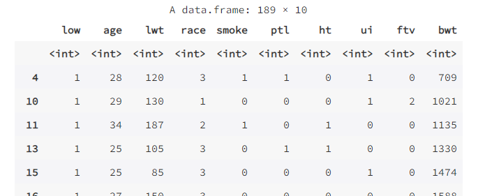
In the above output, the values of the variables bwt in rows 6 and 7 are both 1588. In this case, if you still want to sort the data frames by the second variable, you only need to add the second variable to the function arrange( ). For example, the following command sorts the data frames from small to large according to the value of the variable bwt, and then from small to large according to the value of the second variable age if the values of bwt are equal.
arrange(birthwt, bwt, age)
If you want to sort the data frames by the value of a variable from large to small, you can use the function desc( ).
arrange(birthwt, desc(bwt))
# Identical To
arrange(birthwt, - bwt)
3. Use select () to select columns #
The function select( ) is used to select columns (variables) in a data frame.
# The following command selects the four variables bwt, age, race, and smoke in the data frame to form a new data frame.
select(birthwt, bwt, age, race, smoke)
Note that there is a function with the same name select () in the MASS package. If both the dplyr package and the MASS package are loaded, ** R will default to the function in the later loaded package **. To avoid confusion, we can use the symbol :: to specifically indicate the use of a function in a package, such as dplyr::select( ). After that, we will introduce the function select () further.
4. Add a new variable using mutate () #
The function mutate( ) is used to create a new variable in the data frame. The following command multiplies the variable lwt (unit: lb) in the dataset birthwt by a factor of 0.4536 to generate a new variable lwt.kg (1lb ≈ 0.4536kg).
# Of course, if you want to replace the original variable with the new variable, just name the new variable with the original variable name:
mutate(birthwt, lwt.kg = lwt*0.4536)
5. Use summarise () to calculate statistics #
The function summarise () can be used to calculate a specified statistic for a variable in a data frame.
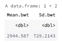
For example, calculate the sample mean and sample standard deviation for the variable bwt:
summarise(birthwt, Mean.bwt = mean(bwt), Sd.bwt = sd(bwt))
6. Split the data frame using group_by () #
Function group_by( ) can split a data frame into multiple data frames according to one or several classification variables. For example:
group_by(birthwt, race)
str(group_by(birthwt, race))

# Output
grouped_df [189 × 10] (S3: grouped_df/tbl_df/tbl/data.frame)
 $ low  : int [1:189] 0 0 0 0 0 0 0 0 0 0 ...
 $ age  : int [1:189] 19 33 20 21 18 21 22 17 29 26 ...
 $ lwt  : int [1:189] 182 155 105 108 107 124 118 103 123 113 ...
 $ race : int [1:189] 2 3 1 1 1 3 1 3 1 1 ...
 $ smoke: int [1:189] 0 0 1 1 1 0 0 0 1 1 ...
 $ ptl  : int [1:189] 0 0 0 0 0 0 0 0 0 0 ...
 $ ht   : int [1:189] 0 0 0 0 0 0 0 0 0 0 ...
 $ ui   : int [1:189] 1 0 0 1 1 0 0 0 0 0 ...
 $ ftv  : int [1:189] 0 3 1 2 0 0 1 1 1 0 ...
 $ bwt  : int [1:189] 2523 2551 2557 2594 2600 2622 2637 2637 2663 2665 ...
 - attr(*, "groups")= tibble [3 × 2] (S3: tbl_df/tbl/data.frame)
  ..$ race : int [1:3] 1 2 3
  ..$ .rows: list<int> [1:3]
  .. ..$ : int [1:96] 3 4 5 7 9 10 15 16 18 20 ...
  .. ..$ : int [1:26] 1 17 29 30 31 33 35 41 43 70 ...
  .. ..$ : int [1:67] 2 6 8 11 12 13 14 19 21 24 ...
  .. ..@ ptype: int(0)
  ..- attr(*, ".drop")= logi TRUE
The function group_by () does not change the appearance of the data frame, but ** changes the way it works with other dplyr verb functions **. Therefore, the above output looks no different from the original data frame, but is essentially different. The most essential difference is that there is one more grouping attribute (Groups), that is, the above result contains 3 data frames, corresponding to the 3 categories of the variable race.
You may also notice the format of the output object above (grouped_df [189 × 10] (S3: grouped_df/tbl_df/tbl/data.frame)). Unlike on R/Rstudio, notebook shows it here as A grouped_df: 189 × 10 (instead of # A tibble: 189 x 10), in fact it still contains tibble (note the - attr(*, "groups")= tibble [3 × 2] (S3: tbl_df/tbl/data.frame) in it). In addition, it does not display the Groups property information, it should actually be # Groups: race [3].
tibble is a data frame-like format provided by the tidyverse family of packages, including the dplyr package. Compared to traditional data frames, tibble has advantages in many ways, and interested readers can refer to the [help document] (https://tibble.tidyverse.org/[1]) of the function tibble (). We can use the function as_tibble( ) to convert a traditional data frame into a tibble, or we can use the function as.data.frame( ) to convert a tibble into a traditional data frame.
as_tibble(birthwt)
Next, we will see that the combination of the functions group_by () and summarise () makes it easy to group variables.
7. Combine multiple actions using the passphrase % > % #
We often need to do a series of operations on a data frame, and the input of the next operation needs to use the output of the previous operation.
# The first step is to convert the variable race in the data frame birthwt into a factor and add labels to each level, and name the new data frame birthwt1
birthwt1 <- mutate(birthwt,
                   race = factor(race, labels = c("white", "black", "other")))
# Step 2: Group the data frame birthwt1 according to the variable race, and name the grouped object birthwt.group;
birthwt.group <- group_by(birthwt1, race)
# Step 3 Calculate the average of the variables bwt in each group for the grouping object birthwt.group.
summarise(birthwt.group, mean(bwt))
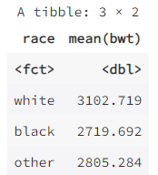
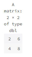
The biggest disadvantage of this approach is the need to establish a variable for each intermediate result. In many cases, such as in the example above, these intermediate variables are actually meaningless. We need to name these intermediate variables, and these intermediate variables are stored in the memory occupied by the workspace. The pass-through operator %>% passes the object preceding the symbol to the function following the symbol as the first parameter value of the function. For example:
c(2, 4, 6, 8) %>% matrix(nrow = 2)
Because the function ** first argument in the dplyr package is always the data frame **, it is very convenient for these functions to handle the data frame with the pass-through operator. The following overrides the above command with the pass-through operator:
birthwt %>%
  mutate(race = factor(race, labels = c("white", "black", "other"))) %>%
  group_by(race) %>%
  summarise(mean(bwt))
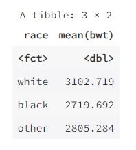
The focus of the above code is on the verb function, not the parameters in the function. When reading this string of code combinations, you can think of them as a set of prescribed actions.
Projects in action #
The data set in the epiDisplay package Planning comes from a family planning survey study in Thailand in the mid-1980s, please use its help file to view the data information and organize the data set.
library(epiDisplay)
data(Planning)
print(des(Planning))

names(Planning) <- tolower(names(Planning))   # Change variable name to lowercase
summary(Planning)

table(duplicated(Planning$id))       # Check if there is a duplicate id;
# FALSE  TRUE
#   250     1
which(duplicated(Planning$id))       # Find the line number of the duplicate id; replace XXXXXX with the correct code
#   216
Planning$id # Under Verification
Planning$id[216] <- 216  # Fix duplicate id;

library(dplyr)
Planning <- mutate(
  Planning,
  relig = ifelse(relig == 9, NA, relig),     # Change 9 in variable relig to NA
  ped = ifelse(ped == 0 | ped == 9, NA, ped), # Change 0 and 9 in variable ped to NA
  income = ifelse(income == 9, NA, income),   # Change 9 of variable income to NA
  am = ifelse(am == 99, NA, am),           # Change 99 in variable am to NA
  reason = ifelse(reason == 9, NA, reason),  # Change 9 in variable reason to NA
  bps = ifelse(bps == 0 | bps == 999, NA, bps), # Change 0 and 999 in variable bps to NA
  bpd = ifelse(bpd == 0 | bpd == 999, NA, bpd), # Change 0 and 999 in variable bpd to NA
  wt = ifelse(wt == 0 | wt > 99, NA, wt),    # Change the value of 0 and greater than 99 in the variable wt to NA
  ht = ifelse(ht == 0 | ht > 300, NA, ht)    # Change the value of 0 and greater than 300 in the variable ht to NA;
)
References
Related readings
If you want to follow my updates, or have a coffee chat with me, feel free to connect with me: