Using Base R

August 17, 2023 · 10 min read

If you have any questions, feel free to comment below. Click the block can copy the code.
And if you think it's helpful to you, just click on the ads which can support this site. Thanks!

Using Base R #

In actual data analysis, analysts often spend a lot of effort on data preparation, transforming data into the form required for analysis. Unfortunately, most statistics textbooks rarely address this important issue. Organizing data is one of the tasks of statistics. We started to focus on the most common data format in R - the basic operation of data frames. We will first process the data frames using the base package.

Load a small dataset Familydata in the epiDisplay package first.

library(epiDisplay)
data("Familydata")

1. See what’s in the data frame #

If the data frame is small, such as this example (only 6 variables, 11 records), just enter the data frame name to view its entire contents, which is equivalent to calling the function print () to display the contents of the object.

# Enter the name of the data frame to see its full contents, which is equivalent to calling the function print () to display the contents of the object.
Familydata
# Show only the first few lines with function `head ()`
head(Familydata)
# Show its last lines with function `tail ()`
tail(Familydata)
# You can specify up to a few rows by adding parameters
tail(Familydata,7) # Show last 7 rows

# List all variable names (column names)
names(Familydata)

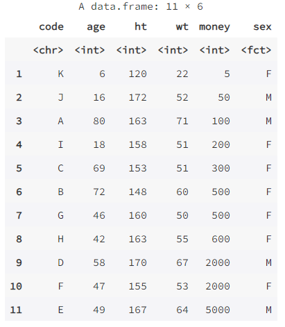
Another function that can be used to easily explore the data frame structure is str( ).

str(Familydata)

# Show results
# First, the type of object (here, the data frame "data.frame"), the number of observations and the number of variables are given;
'data.frame':	11 obs. of  6 variables:
# Then give the variable name and type of each variable in the data frame, as well as the first few values of the variable
 $ code : chr  "K" "J" "A" "I" ...
 $ age  : int  6 16 80 18 69 72 46 42 58 47 ...
 $ ht   : int  120 172 163 158 153 148 160 163 170 155 ...
 $ wt   : int  22 52 71 51 51 60 50 55 67 53 ...
 $ money: int  5 50 100 200 300 500 500 600 2000 2000 ...
 # The level of the factor is also given for factor-type variables;
 $ sex  : Factor w/ 2 levels "F","M": 1 2 2 1 1 1 1 1 2 1 ...
 # Finally, some properties of the data frame are given:
 # Data Label (“datalabel”)
 - attr(*, "datalabel")= chr "Anthropometric and financial data of a hypothetical family"
 - # Data creation time ("time.stamp")
 - attr(*, "time.stamp")= chr "23 Nov 2006 17:15"
 - attr(*, "formats")= chr [1:6] "%9s" "%8.0g" "%8.0g" "%8.0g" ...
 - attr(*, "types")= int [1:6] 128 98 105 98 105 108
 # Variable labels ("var.labels")
 - attr(*, "val.labels")= chr [1:6] "" "" "" "" ...
 - attr(*, "var.labels")= chr [1:6] "" "Age(yr)" "Ht(cm.)" "Wt(kg.)" ...
 # Version number
 - attr(*, "version")= int 7
 - attr(*, "label.table")=List of 6
  ..$ sex1: Named num [1:2] 1 2
  .. ..- attr(*, "names")= chr [1:2] "F" "M"
  ..$     : NULL
  ..$     : NULL
  ..$     : NULL
  ..$     : NULL
  ..$     : NULL

These properties can enhance the user’s understanding of the dataset. To display all information about the data frame properties, you can use the attributes( ) function, whose output is a list.

attributes(Familydata)
# Output
$names
'code''age''ht''wt''money''sex'
$row.names
1234567891011
$class
'data.frame'
$datalabel
'Anthropometric and financial data of a hypothetical family'
$time.stamp
'23 Nov 2006 17:15'
$formats
'%9s''%8.0g''%8.0g''%8.0g''%8.0g''%8.0g'
$types
1289810598105108
$val.labels
'''''''''''sex1'
$var.labels
'''Age(yr)''Ht(cm.)''Wt(kg.)''Pocket money(B.)'''
$version
7
$label.table
$sex1
F1M2
[[2]]
NULL
[[3]]
NULL
[[4]]
NULL
[[5]]
NULL
[[6]]
NULL

These properties can also be modified and customized. For example, as you can see from the output above, the first variable and the last variable do not have a label defined. Now add tags for these two variables:

attr(Familydata, "var.labels")[1] <- "Identification number"
attr(Familydata, "var.labels")[6] <- "Gender"
attributes(Familydata)$var.labels
# 'Identification number''Age(yr)''Ht(cm.)''Wt(kg.)''Pocket money(B.)''Gender'

Labeling variables helps us better understand what they mean. In addition, the output of some functions in the epiDisplay package used later can also use these variable labels directly.

2. Select a subset of the data frame #

Similar to a matrix, we can select a subset of data frames by index subscripts.

# Select column 3 of the data frame Familydata
Familydata[, 3]
# You can also use the $ variable name
Familydata$ht

# To extract more than one variable, you can use the index number or name of the variable. For example, to display only the first 3 records for the variables ht, wt, and sex, you could enter:
Familydata[1:3, c(3, 4, 6)]
# Identical To
Familydata[1:3, c("ht", "wt", "sex")]

An index in a subscript can also be a conditional statement. For example, to select data where gender is female, you could enter:

Familydata[Familydata$sex == "F", ] # Note commas and double equals signs

Another way to select a subset of a data frame is to use the subset( ) function.

subset(Familydata, sex == "F")
# If only the variables ht and wt in women are selected
subset(Familydata, sex == "F", select = c(ht, wt))

** Note that this command only selects a subset to display and will not have any effect on the original data frame. If you want to use this subset further, you need to save it as a new object. **

In the field of machine learning, it is often necessary to take a random sample from a dataset. For example, we want to randomly divide a large dataset into two parts, one for building the prediction model and the other for verifying the prediction accuracy of the model. The function sample( ) can be used for random sampling, and the following command randomly extracts a sample of size 3 from the data frame Familydata:

sample.rows <- sample(1:nrow(Familydata), size = 3, replace = FALSE)
sample.rows
# 5 4 1

The first parameter in the function sample () is a vector consisting of the elements to be sampled from, here is the total number of observations from 1 to the data frame; the second parameter size is the number of elements to be sampled; the third parameter replace is used to set whether to play back the sampling, the default is false (no playback sampling).

The return value of the function sample () can be used to select rows in the data frame. Due to the different number of random seeds, the results are likely to be different for each run.

3. Sort the data frames by the value of a variable: order () #

Sometimes we want to sort the data frames by the size of a variable’s value, which can be achieved with the help of the function order( ). For example, to display the data frame Familydata with the value of the variable age from small to large, you can use the following command:

# , front indicates condition, back indicates displayed column
Familydata[order(Familydata$age), ] # Default ascending
# Descending Writing
Familydata[order(Familydata$age, decreasing = TRUE), ]
# Equivalent to age Negating Result
Familydata[order(-Familydata$age), ]

4. Find and deduplicate data: duplicated () #

There are often duplicate rows in the original dataset. If the data is not repeatedly measured, each row of the dataset should be an observation of an object, and there is usually a variable (such as id) in the dataset that identifies the individual.

The variable code in the dataset Familydata is the individual identification number, and the following checks whether the variable has duplicate values:

duplicated(Familydata$code)
# FALSE FALSE FALSE FALSE FALSE FALSE FALSE FALSE FALSE FALSE FALSE
# The return value of the function duplicated () is the logical value true or false, which is all FASLE, indicating that the variable code does not have a duplicate value.

If the data frame has a large number of rows, it can be cumbersome to look at these logical values one by one. At this point, you can apply the function any( ) to the output of the function duplicated ():

any(duplicated(Familydata$code))
# FALSE

Or use the function table( ) to get the number of duplicate values:

table(duplicated(Familydata$code))
# FALSE 
# 11

Delete Dulicate Rows

To illustrate how to remove duplicate rows, create a data frame Familydata1 below and add the second row of the original data frame Familydata to its 12th row:

Familydata1 <- Familydata
Familydata1[12, ] <- Familydata[2, ]
Familydata1

Use the function which( ) to find the row where the duplicate value of the variable code is located:

which(duplicated(Familydata1$code))

Then, delete the duplicate rows:

# Just create a new object with no duplicates
unique.code.data <- Familydata1[!duplicated(Familydata1$code), ]
unique.code.data

identical Check if the objects are exactly the same

# Use identical to see if the two objects are exactly the same
identical(unique.code.data, Familydata)
# TRUE

5. Adding and removing variables in data frames #

When working with data frames, we often need to create new variables and add them to existing data frames. For example, create a new variable log10money whose value is equal to the logarithm of the variable money with base 10. Most directly, you can enter:

Familydata$log10money <- log10(Familydata$money)
# Or you can use the `transform ()` function:
Familydata <- transform(Familydata, log10money = log10(money))
names(Familydata)
# 'code''age''ht''wt''money''sex''log10money'

As opposed to adding variables, if you want to remove a variable from the data frame, just add a minus sign ** before the ** subscript in square brackets. For example:

Familydata[, -7]

Note that ** this command displays only the desired subset and does not affect the data frame itself. **

But assigning a null value to a variable in a data frame is equivalent to deleting the variable, and is a variable that permanently deletes the data frame:

Familydata$log10money <- NULL
colnames(Familydata)

6. Add the data frame to the search path #

When viewing and using the variables in the data frame in front, we need to prefix the variable name with the data frame name and the symbol $. This can sometimes seem cumbersome, especially when the data frame and variable names are long. At this point, the function attach( ) or the function with( ) can be used to simplify the code.

Function attach( ) can ** add data frames to the search path **. Enter the following command:

attach(Familydata)

Then use the function search( ) to view all objects in the search path:

search()
#'.GlobalEnv''Familydata''package:epiDisplay''package:nnet''package:MASS''package:survival''package:foreign''package:repr''jupyter:irkernel''package:stats''package:graphics''package:grDevices''package:utils''package:datasets''package:methods''Autoloads''package:base'

The second location in the search path now holds the data frame Familydata. Since the ** data frame is already in the search path and the variable age is in the data frame, you can now use the variable age directly. **

summary(age)
#    Min. 1st Qu.  Median    Mean 3rd Qu.    Max. 
#    6.00   30.00   47.00   45.73   63.50   80.00

Putting a data frame into the search path is similar to loading a package with the function library (). The data frames in the search path and the loaded packages are automatically read into R and stored in memory until they are removed (detach( )).

Using the function attach( ) brings some convenience when entering code, but it also brings some problems. For example, repeatedly loading data frames may eventually lead to overloading of system resources. In addition, it is easy to confuse users if there are the same variable names in the global environment or in multiple data frames. Therefore, some users of R ** try to avoid using the function attach () and instead use the function with( ). **

Take the data set infert in the datasets package as an example:

with(infert, summary(age))
#  Min. 1st Qu.  Median    Mean 3rd Qu.    Max. 
#  21.00   28.00   31.00   31.50   35.25   44.00

The limitation of the function with () is that for using the data frame multiple times, we have to reuse the function with (). In addition, the assignment only takes effect within this function, for example:

with(infert, {
  m <- mean(age)}
  )
m 
# ERROR：object 'm' not found

Which data processing method to choose depends on the analyst’s preferences. For example, the R Language Medical Data Analysis Practice recommends:

When starting a new analysis project, first use the command rm(list = ls( )) to clear all objects from the R working environment;
In the process of analysis, use the function detach( ) to remove the data frames that are no longer needed from the search path;
Do not define a new object with the same name as a data frame that already exists in the search path;