Data Structures and Conversion
August 16, 2023 · 11 min read
If you have any questions, feel free to comment below. Click the block can copy the code.
And if you think it's helpful to you, just click on the ads which can support this site. Thanks!
The first step in any data analysis is to create a dataset in the required format. In R, this task consists of two steps: first select a data structure to store the data, and then enter or import the data into this data structure. The following introduces the various data structures used to store data in R.
R Data Structures #
- In most cases, structured data is a dataset composed of many rows and many columns. In R, this kind of dataset is called a data frame.
- Before learning about data frames, let us first get to know some data structures used to store data: vectors, factors, matrices, arrays, and lists.
1.1 Vectors #
A vector is a one-dimensional array used to store numeric, character, and logical data. A scalar can be regarded as a vector containing only one element. The function c( ) can be used to create vectors, for example:
x1 <- c(2, 4, 1, -2, 5)
x2 <- c("one", "two", "three")
x3 <- c(TRUE, FALSE, TRUE, FALSE)
Here x1 is a numeric vector, x2 is a character vector, and x3 is a logical vector. The data type within each vector must be consistent. If you want to create a vector with a pattern, R provides some convenient operations and functions, for example:
x4 <- 1:5     # Equivalent to x4 <- c(1, 2, 3, 4, 5)
x5 <- seq(from = 2, to = 10, by = 2)  # Equivalent to x5 <- c(2, 4, 6, 8, 10)
x6 <- rep("a", times = 4)  # Equivalent to x6 <- c("a", "a", "a", "a")
Sometimes we only want to use a certain part of a vector, that is, select a subset of the vector. Suppose there is an integer vector from 3 to 100 with a step size of 7; what is the value of the 5th number?
x <- seq(from = 3, to = 100, by = 7)
# Display the 5th element
x[5]
# Display the 4th, 6th, and 7th elements
x[c(4, 6, 7)]
The numbers in square brackets “[ ]” are called subscripts, and they specify the index positions of the vector. In the command above, x[5] represents the 5th element of the vector, whose value is 31.
The vector in the subscript can take negative values, indicating the removal of elements at specified positions. For example, to remove the first 4 elements of x, you can enter the following code (note the parentheses in the command):
x[-(1:4)]
Operations in R are vectorized, for example:
weight <- c(68, 72, 57, 90, 65, 52)
height <- c(1.75, 1.80, 1.65, 1.90, 1.72, 1.65)
bmi <- weight / height ^ 2
bmi
In the process of calculating bmi above, the operator “^” was used cyclically, so the result of the calculation is still a vector. If the lengths of the vectors participating in the operation are inconsistent, R will automatically complete them before calculating. The completion rule is to cycle the shorter vector, while also issuing a warning message.
a <- 1:5
b <- 1:3
a + b
# Warning message in a + b:
# “longer object length is not a multiple of shorter object length”
# 2 4 6 5 7
Common Statistical Functions #
| Function | Description |
|---|---|
| length(x) | Find the number of elements in x |
| mean(x) | Find the arithmetic mean of x |
| median(x) | Find the median of x |
| var(x) | Find the sample variance of x |
| sd(x) | Find the sample standard deviation of x |
| range(x) | Find the range of x |
| min(x) | Find the minimum value of x |
| max(x) | Find the maximum value of x |
| quantile(x) | Find the quantiles of x |
| sum(x) | Find the sum of all elements in x |
| scale(x) | Standardize x |
1.2 Factors #
Generally speaking, variables are divided into numeric, nominal, and ordinal types.
Nominal variables are categorical variables with no ordering relationship, such as a person’s sex, blood type, ethnicity, and so on. Ordinal variables are categorical variables with hierarchical and ordering relationships, such as a patient’s condition (poor, improved, excellent). Nominal variables and ordinal variables are called factors in R.
Factors are very important in R; they determine how data are displayed and analyzed. When data are stored, factors are often stored in the form of integer vectors. Therefore, before performing data analysis, it is often necessary to convert them into factors with the function factor( ).
# First define a variable sex representing sex, assuming that its value 1 represents male and 2 represents female.
sex <- c(1, 2, 1, 1, 2, 1, 2)
# Next, use the function factor( ) to convert the variable sex into a factor and store it as the object sex.f, where the parameter levels represents the category label values of the original variable, and the parameter labels represents the labels of the factor values.
sex.f <- factor(sex,
                levels = c(1, 2),
                labels = c("Male", "Female"))
sex.f
# ============ Output =============
# Male Female Male Male Female Male Female
# **Levels**:
# 'Male''Female'
Note that these two parameters need to correspond one-to-one when assigned, and R will associate them. The difference between a factor variable and an ordinary character variable is that it has a level attribute. The attributes of a factor can be viewed using the function levels( ):
levels(sex.f)
# 'Male''Female'
Changing the Order of Factor Levels → Changing the Reference Group #
In statistical models, for a factor variable, R treats its first level as the reference group. Often we need to change the order of factor levels to change the reference group, which can be achieved in two ways. The first method is to change the order of the parameters levels and labels in the function factor( ), for example:
sex.f1 <- factor(sex, levels = c(2, 1), labels = c("Female", "Male"))
sex.f1
# Male Female Male Male Female Male Female
# **Levels**:
# 'Female' 'Male'
The second method is to use the function relevel( ):
sex.f1 <- relevel(sex.f, ref = "Female")
sex.f1
# Male Female Male Male Female Male Female
# **Levels**:
# 'Female' 'Male'
Ordinal Factors: ordered = TRUE #
To represent an ordered factor, you need to specify the parameter ordered = TRUE in the function factor ( ). For example:
status <- c(1, 2, 2, 3, 1, 2, 2)
status.f <- factor(
  status,
  levels = c(1, 2, 3),
  labels = c("Poor", "Improved", "Excellent"),
  ordered = TRUE
)
status.f
# PoorImprovedImprovedExcellentPoorImprovedImproved
1.3 Matrices #
A matrix is a two-dimensional array composed of rows and columns. Every element in a matrix has the same mode (numeric, character, or logical). In most cases, the elements in a matrix are numeric. It has many mathematical properties and operations and can be used for statistical calculations, such as factor analysis, generalized linear models, and so on.
1.3.1 Creation: matrix( ) #
The function matrix( ) is commonly used to create matrices, for example:
M <- matrix(1:6, nrow = 2)
M
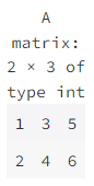
R automatically calculates the number of columns based on the length of the vector and the number of rows set by the parameter nrow. The parameter byrow defaults to FALSE, meaning that values are arranged by column; if you need to arrange by row, simply set the parameter byrow to TRUE.
Common matrix operations can all be implemented in R, such as matrix addition, matrix multiplication, finding an inverse matrix, matrix transposition, finding the determinant of a square matrix, and finding the eigenvalues and eigenvectors of a square matrix.
1.3.2 Multiplication: %*% #
Matrix multiplication requires that the number of columns in the first matrix equal the number of rows in the second matrix, and its operator is %*%.
First create two matrices:
mat1 <- matrix(1:6, nrow = 3)
mat1
mat2 <- matrix(5:10, nrow = 2)
mat2
# The function dim( ) can obtain the dimensions of a matrix, namely the number of rows and columns
dim(mat1)
# 32
dim(mat2)
# 23
mat1 %*% mat2
1.3.3 Transposition: t( ) #
The transpose operation of a matrix interchanges the rows and columns of the matrix. For example, find the transpose of matrix mat1:
t(mat1)
1.3.4 Determinant and Inverse Matrix: det( ), solve( ) #
The determinant and inverse matrix of a square matrix can be obtained using the functions det( ) and solve( ), respectively. For example:
mat3 <- matrix(1:4, nrow = 2)
det(mat3)
# -2
1.3.5 Sum or Average by Row or Column: rowSums, colSums, rowMeans, ColMeans #
For example:
rowSums(mat1)
colSums(mat1)
rowMeans(mat1)
colMeans(mat1)
1.4 Arrays #
What is commonly called an array refers to a multidimensional array. It is similar to a matrix, but its number of dimensions is greater than 2. An array has a special dimension (dim) attribute.
The following command defines an array by adding dimensions to a vector; please note the order in which the values are arranged.
Because arrays do not display very nicely in the notebook, it is recommended to use
print(). The following code will additionally add print() when displaying arrays.
A <- 1:24
dim(A) <- c(3, 4, 2)
# A # Arrays do not display very normally in the notebook; using print() can solve this
print(A)
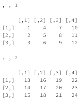
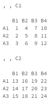
The array above can also be created with the function array( ), and names and labels can be added to each dimension.
dim1 <- c("A1", "A2", "A3")
dim2 <- c("B1", "B2", "B3", "B4")
dim3 <- c("C1", "C2")
print(array(1:24, dim = c(3, 4, 2), dimnames = list(dim1, dim2, dim3)))
1.5 Lists #
A list is the most flexible and complex data structure in R, and it can consist of a mixture of different types of objects. For example, it can be a combination of vectors, arrays, tables, and objects of any type.
list1 <- list(a = 1, b = 1:5, c = c("red", "blue", "green"))
list1
# $a
# 1
# $b
# 1 2 3 4 5
# $c
# 'red''blue''green'
In ordinary data analysis, creating lists is not a common task. The return values of many functions are lists. For example:
# To make the results reproducible, we use the function set.seed( ) before this command to set the seed for generating random numbers. If the seed is not set, the results displayed each time are likely to differ.
set.seed(123)
# Use the function rnorm( ) to generate a random sample consisting of 10 numbers from the standard normal distribution.
dat <- rnorm(10)
# Use the function boxplot( ) to make a **box plot** of this random sample, and save the result as bp.
bp <- boxplot(dat)
# The function class( ) is used to view the type of an object; here bp is a list.
class(bp)
# 'list'
View the contents of this list:
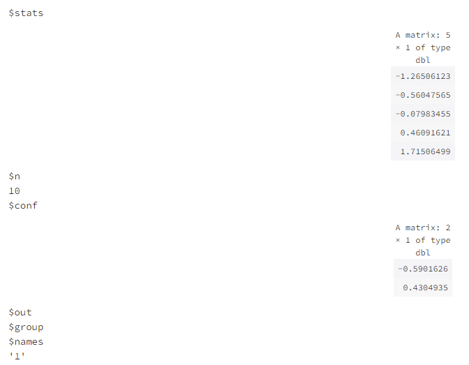
Here the list bp contains multiple objects. If you want to view or use one of the objects, simply reference it with the “$” symbol. For example, to view the contents of the object stats in the list bp, you can enter bp$stats. If you are interested in other objects in the list, please proceed to the documentation[1] for boxplot.stats.
1.6 Data Frames #
A data frame is a two-dimensional structure composed of rows and columns, where rows represent observations or records, and columns represent variables or indicators. A data frame is similar to datasets in Excel, SAS, and SPSS. A data frame looks very similar to a matrix, and many matrix operations also apply to data frames, such as subset selection.
Unlike a matrix, different columns in a data frame can contain data of different modes (numeric, character, and so on). A data frame can be created with the function data.frame( ). For example, the following code creates a data frame containing 5 observed objects and 4 variables:
ID <- 1:5
sex <- c("male", "female", "male", "female", "male")
age <- c(25, 34, 38, 28, 52)
pain <- c(1, 3, 2, 2, 3)
pain.f <- factor(pain, levels = 1:3, labels = c("mild", "medium", "severe"))
patients <- data.frame(ID, sex, age, pain.f)
patients
A data frame is essentially also a type of list. To display or use a variable (column) of a data frame, you can use the $ symbol followed by the variable name. For example:
patients$age
mean(patients$age)
Most structured medical datasets are presented in the form of data frames; therefore, data frames are the most commonly processed data structure.
Data Type Conversion: is., as. #
When performing data analysis, analysts need to know the types of data thoroughly, because the choice of data analysis method is closely related to the type of data. R provides a series of functions for determining the data type of an object, and also provides functions for converting one data type into another data type. These functions all exist in the base package; some of the commonly used functions are listed below:
Data Type Determination and Conversion Functions #
| Determination | Conversion |
|---|---|
| is.numeric( ) | as.numeric( ) |
| is.character( ) | as.character( ) |
| is.logical( ) | as.logical( ) |
| is.factor( ) | as.factor( ) |
| is.vector( ) | as.vector( ) |
| is.matrix( ) | as.matrix( ) |
| is.array( ) | as.array( ) |
| is.data.frame( ) | as.data.frame( ) |
| is.list( ) | as.list( ) |
| is.table( ) | as.table( ) |
Functions beginning with is. return TRUE or FALSE, while functions beginning with as. convert an object to the corresponding type. For example:
x <- c(2, 5, 8)
is.numeric(x)
# TRUE
is.vector(x)
# TRUE
y <- as.character(x)
y
# '2''5''8'
is.numeric(y)
# FALSE
is.character(y)
# TRUE
z <- c(TRUE, FALSE, TRUE, FALSE)
is.logical(z)
# TRUE
as.numeric(z)
# 1 0 1 0
Reference: Zhao Jun, Practical Medical Data Analysis with R[2]
References
Related readings
If you want to follow my updates, or have a coffee chat with me, feel free to connect with me: